1 Week 1
2 Summary
2.1 What is remote sensing?
Remote sensing is a subset of Geographic Information Science (GIS). Broadly, it refers to the science (and art) of using remote instruments – sensors mounted on satellites or planes – to record information remotely. This week, I will cover some sources of remote sensing data, as well as some applications of its use.
2.2 Active and passive sensors
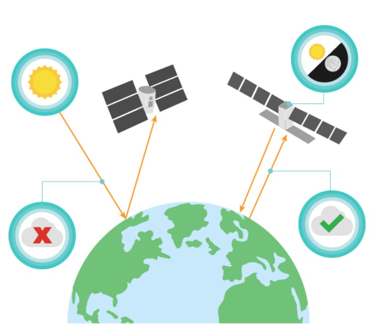
There are two key types of remote sensors: Passive and active. Passive sensors read light from the sun reflected off the earth’s surface. The images they read can be interfered with by, for example, clouds or atmospheric haze. Active sensors, on the other hand, send a signal down to the earth that bounces back to the satellite’s sensor. These sensors can, as a result, operate at night and see through clouds. The figure below illustrates the difference:
2.2.1 Electromagnetic signatures
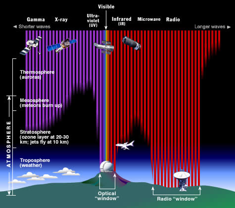
As discussed above, passive sensors read radiation reflected from the earth’s surface. Different types of radiation have different wavelengths, and operate in different parts of the electromagnetic spectrum. And different materials reflect different values on different parts of the electromagnetic spectrum. So different sensors can read different wavelengths, which provide different types of information (and operate under different constraints).
The figure below shows the electromagnetic spectrum, and different instruments that operate at different points on the spectrum. The earth’s atmosphere blocks most wavelengths on the spectrum, with the exceptions of radio waves, visible light (the ‘optical window’ below), and some parts of the infrared spectrum. Most passive sensors read wavelengths within the optical window, and active sensors operate using radio waves.
2.2.2 Resolutions
Remote sensing data has four resolutions, namely:
Spectral: The number of bands that the sensor records (for example, red, green, blue for visible light).
Spatial: The size of each pixel (this can go down to centimetres for very high resolution data or be up to over a kilometre for some purposes).
Temporal: The frequency with which a given area will be revisited (there is often a tradeoff between spatial and temporal resolution, as a lower spatial resolution allows for more of the earth’s surface to be captured and hence a higher temporal resolution).
Radiometric: The range of reflectance values.
3 Applications
In my view, the most exciting applications for remote sensing data are in situations where traditional forms of data collection – such as a national census – are unreliable or out of date. This is true of South Africa, where obtaining up-to-date demographic or economic information is very difficult. I’ll discuss that a bit more in week 4, when I get into policy.
There are many applications of Remote Sensing, and they tend to overlap quite a bit, but since the practical covered imagery from Sentinel 2 and Landsat 8, I’ll cover some interesting applications of these two sources of imagery here:
3.0.1 Sentinel 2
The main advantage of Sentinel 2 over Landsat 8 is its higher resolution (across most bands, it has higher spatial resolution, its revisit time is shorter, and it has more spectral bands). However, Landsat 8 has thermal infrared bands, which means that it can be used to measure temperature.
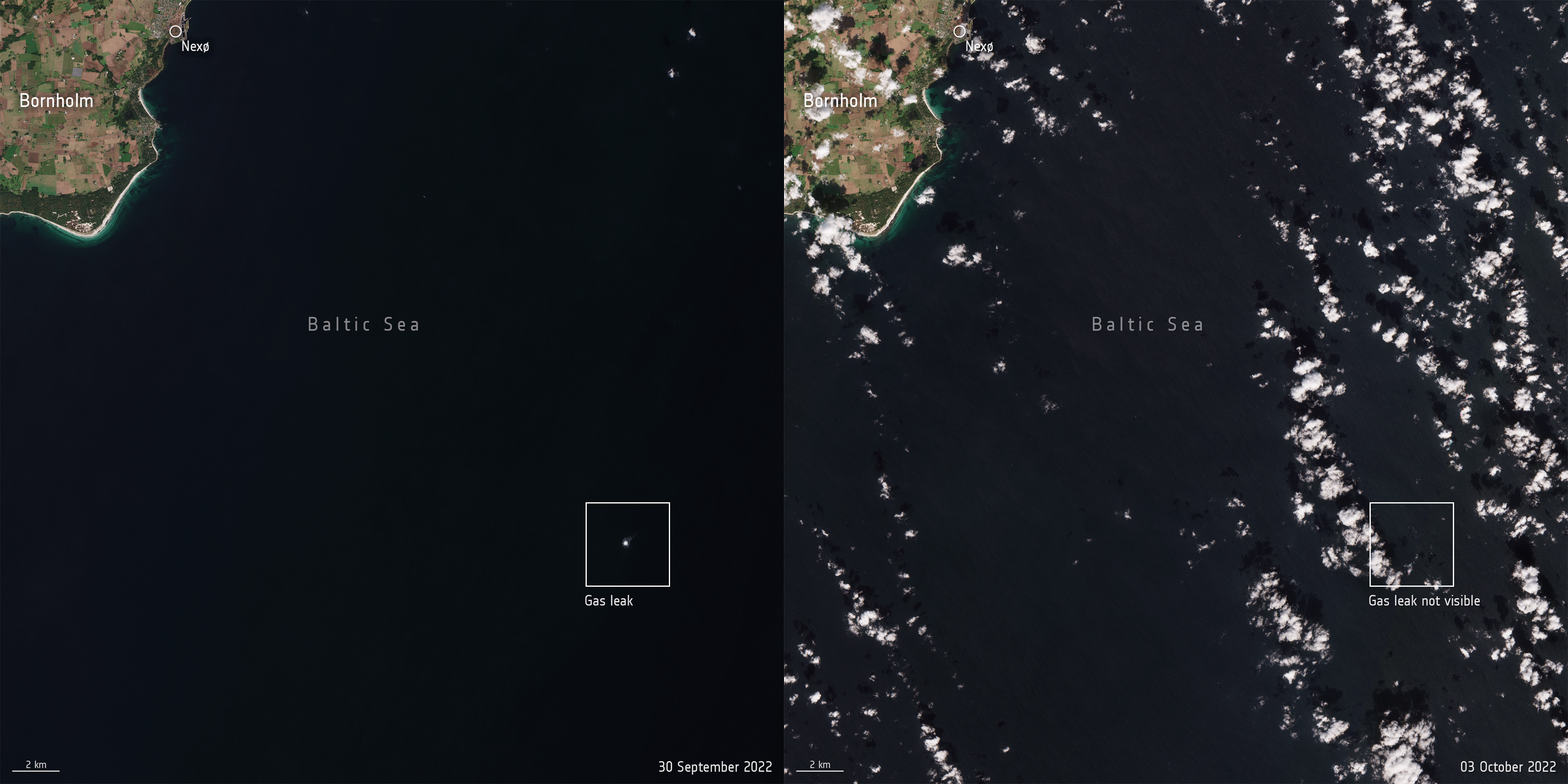
One interesting recent application of Sentinel-2 was when it was used to detect a gas leak in the Nord Stream pipeline following seismic disturbances. Here’s an animation showing the gas leak appearing:
It can also be used for monitoring sea ice, as this (very promotional) video shows – just watch the part between 2 and 3 minutes:
The temporal and spatial resolution of sentinel-2 makes it possible to monitor individual glaciers and see how they interact with the oceans around them. Pretty exciting!
3.0.2 Landsat
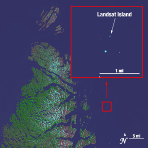
Landsat has been around for more than 50 years now – the first Landsat satellite went up in 1972. One of the earliest applications of Landsat was ‘discovering’ a previously uncharted island off the coast of Canada (it’s possible the island had been discovered previously but not documented). Today the island is called Landsat Island, after its ‘discoverer’.
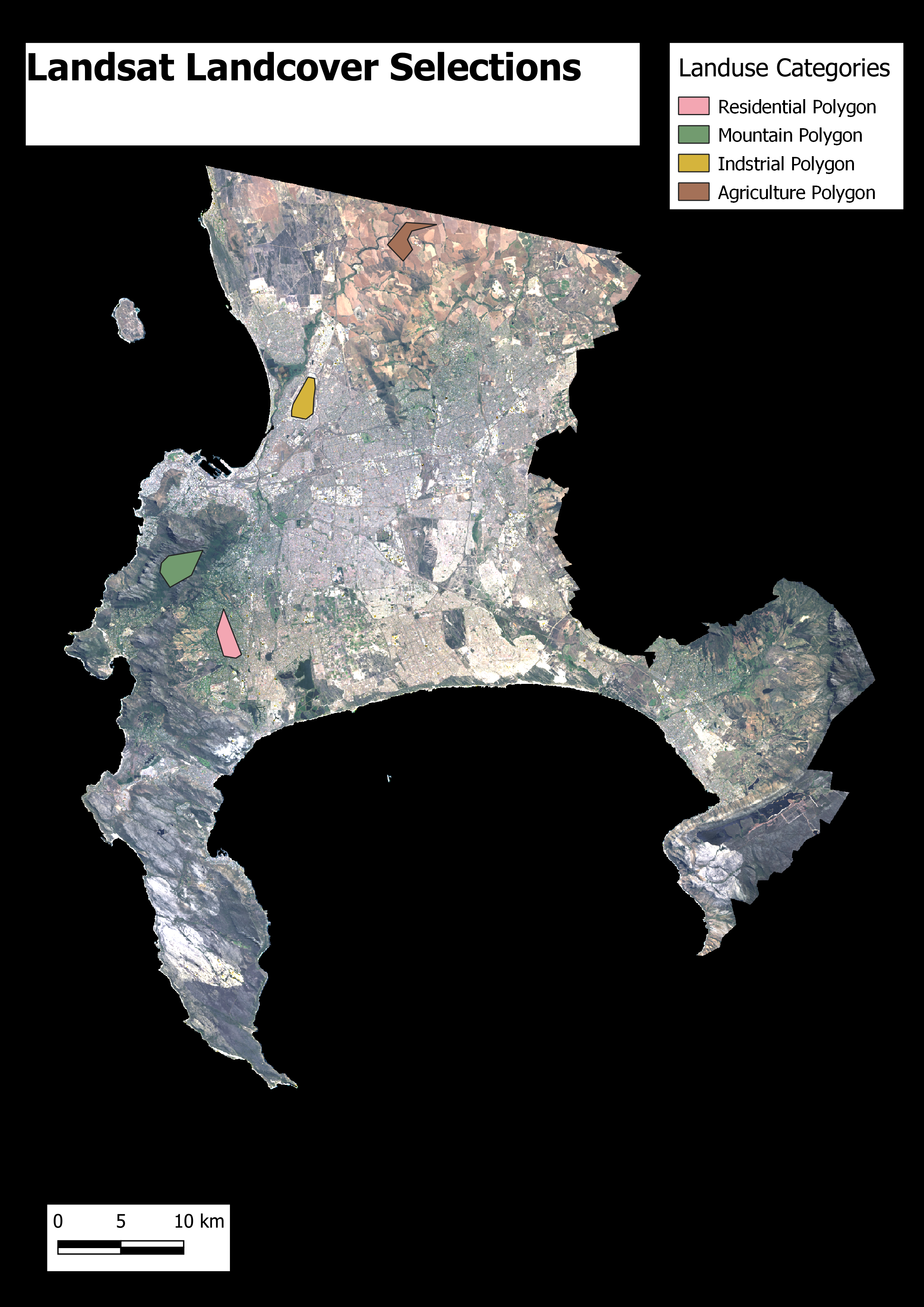
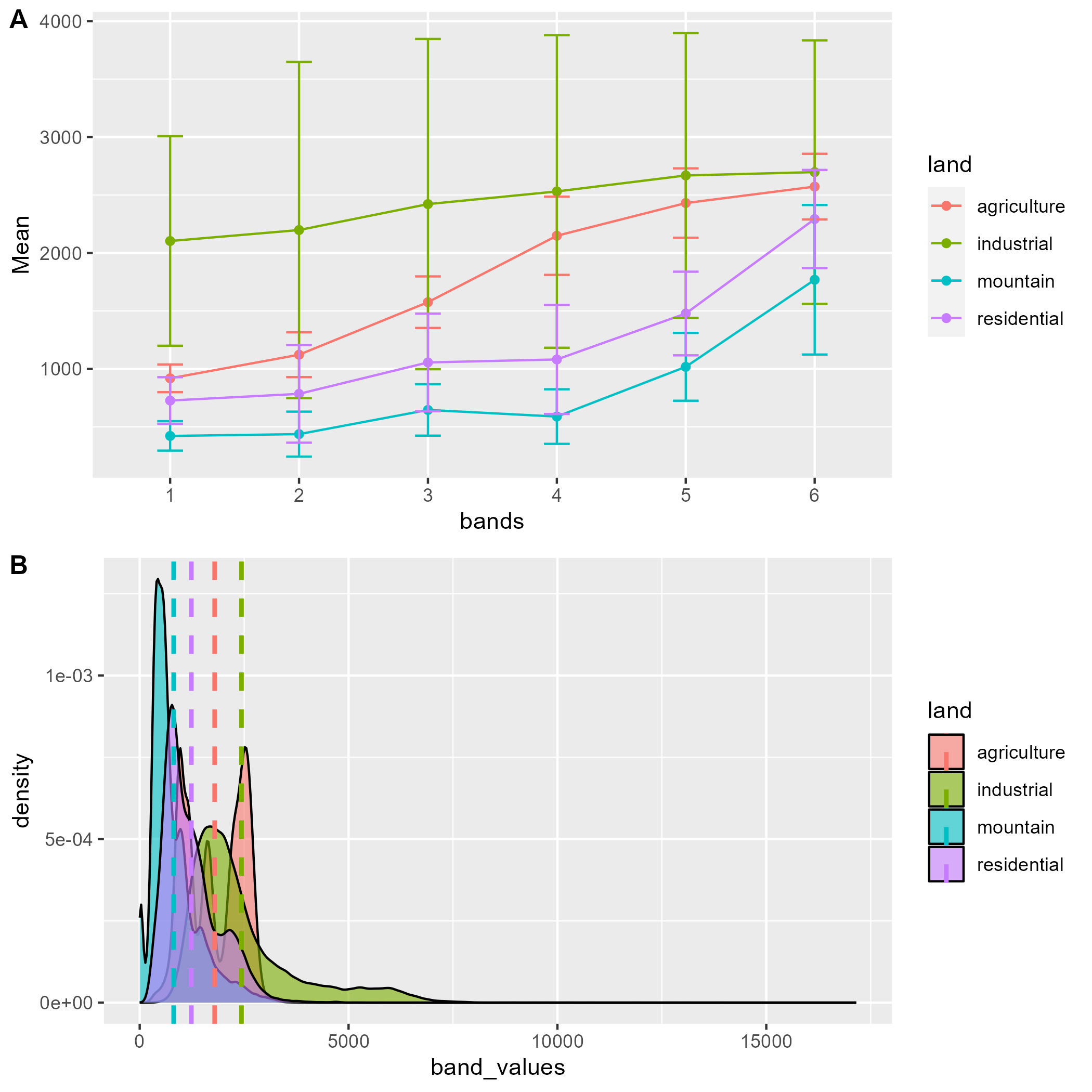
Today, both Landsat 8 and 9 are operational. Here’s my very rudimentary application of Landsat data: I built a true-colour composite from the red, green and blue bands, selected some areas in Cape Town, and plotted their spectral signatures in R. Here’s the composite and areas I selected:
And here are the spectral values of the areas plotted in R:
3.1 Reflections
My first impression was how long a lot of this takes. Working with the raster data in SNAP and then processing it in R is time consuming and convoluted – and it made me look forward to getting into Google Earth Engine later in the term. It’s also just a totally new approach to looking at imagery compared to what I am used to, which feels both exciting and unfamiliar.
I’ve got experience in photography from my previous career, so it was also interesting to interact with large raster files in a completely different way, and to play around with histograms from the electromagnetic spectrum (my previous exposure to histograms and raster imagery was in trying to get rid of ‘clipping’ in areas of a photograph that are over-or-under exposed – which means that parts of an image are entirely black or white. Working with the images in SNAP and then displaying them in QGIS reminded me of that). It’s also quite cool to see how an image can be ‘built’ from three greyscale RGB bands into a full colour composite – it helped me to better understand how digital images are really just data.
I’m also quite used to using satellite imagery as a basemap for spatial analysis in my other previous job as an urban planner. There, the purpose was usually to provide context for the viewer looking at the map (or for myself when working). That was often quite high resolution RGB imagery, and I took it for granted that I was able to zoom into a particular location and see what was happening at a very fine scale. It’s quite interesting to change tack here to working with spectral imagery, which has a lower resolution but a lot more information because of the different bands. I’m looking forward to the rest of the module, and learning a whole lot more.